Gradient Descent Intuitively Understood

Gradient Descent is one of many wildly used optimization algorithms. It’s built on measuring the change of a function with respect to the parameter.There are other variants that extend the vanilla version of Gradient Descent and performs better than it. But a good understanding of it is important to begin with.

Measure The Rate of Change

The learning process is in other words an optimization process. To begin on what gradient descent is and how it works, it is extremely useful to hang onto this part of math started by Isaac Newton:

Suppose this is a function that represents our problem:

This is the derivative of that function:

It makes things much easier to realize that derivative is a way of measuring the rate of change of the function (with respect to the variable). This realization helps simplify the symbol form of this math into the understanding that will pave your way out to grasp several complicated algorithms in the future(e.g., backward propagation).

The function we had above has only one variable. In problems that many machine learning algorithms are solving, one can have a few to millions of variables:

It will come the time that you need to measure the rate of the change of the function with respect to one single variable, this measure using the derivative is called the partial derivative. It is just the normal derivative taken with respect to one variable while considering all the rest of the variables constants.

In [1]:

# the plot setup
%pylab inline
#import mpld3
#mpld3.enable_notebook()
import matplotlib.pyplot as plt
from pylab import rcParams

from contextlib import contextmanager

@contextmanager
def zoom_plot(w, h):
    '''
    Temprarily change the plot size.
    '''
    shape = rcParams['figure.figsize']
    rcParams['figure.figsize'] = w, h
    yield
    rcParams['figure.figsize'] = shape

Populating the interactive namespace from numpy and matplotlib

In [2]:

import numpy as np

def f(x):
    return x**2

def derivative_f(x):
    return 2*x

def tangent_line(x):
    return lambda x_: f(x) - derivative_f(x) * (x - x_)

def plot_derivative():
    # Draw the object function
    X = np.arange(-100, 100, 1)
    Y = np.apply_along_axis(f, 0, X)
    plot(X, Y, '-b')
    # Draw the tangent line
    _X = [-50, -20, 20, 50]
    _Y = list(map(f, _X))
    plot(_X, _Y, 'ob')
    lines = map(tangent_line, _X)
    for (n, line) in zip(_X, lines):
        _x = np.arange(n-30, n+30, 1)
        _y = list(map(line, _x))
        plot(_x, _y, '-k')
    plt.grid(True)
    plt.title("The tangent line at x positions")
    plt.show()

with zoom_plot(4, 4):
    plot_derivative()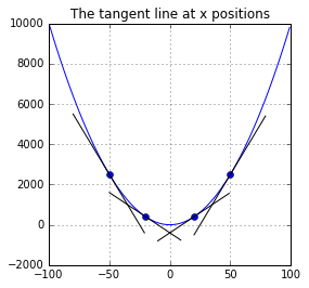

png

The plot above shows the tangent line at the four positions on the defined function.

Given one function:

The tangent line function at position (x, y) is given by:

The tangent line gives us much information about that position:

whether the change is increasing or decreasing
how fast it increases or decreases

(In fact, the second derivative will reveal even more information to us, such as the existance of a local minimum in a certain range of the function. This property is better studied as convexity.)

The cost definition

A cost function is one that describes the quality of the prediction of the model. An MSE, or Mean Squared Error measures the average differences between the predictions and the actual output given one training data set:

In [3]:

# Our model definition
import numpy as np


class LinearModel(object):
    
    def __init__(self, weights):
        self.weights = weights
        self.dimension = len(weights)
    
    def predict(self, X):
        return np.dot(X, self.weights)
    
    def cost(self, X, Y):
        '''
        Measuring the Mean Squared Error over the training set.
        '''
        return np.mean(np.power(np.dot(X, self.weights) - Y, 2))

Utilizing the information revealed by that derivative (slope of the tangent line) we can decide how to move the x so that the function converges to a local minimum:

In the equation above, the λ is an added control on the size of the step, also called the learning rate, and here below is a direct translation of that observation into our gradient descent algorithm:

In [4]:

def gd(model, X, Y, cost_derivative, rate=0.1, epoch=100):
    '''
    The batch gradient descent.
    
    cost_derivative
        callable, calculates the partial derivative of
        the cost with respect to the weight.
    
    epoch
        int, default generations to run the GD before yielding.
    '''
    converged = False
    num_generations = 0
    distance = epoch # num of iterations to run before yielding
    while not converged:
        changes = cost_derivative(model, X, Y)
        weights_updated = (model.weights - rate * changes) # resize the step
        converged = (weights_updated == model.weights).all()
        model.weights = weights_updated
        distance -= 1
        num_generations += 1
        if distance == 0: # reached checkpoint
            # allows the outside to change rate
            control = yield (converged, num_generations, rate, epoch)
            if control: rate, epoch = control
            distance = epoch # reset the distance
    yield (converged, num_generations, rate, epoch)
    raise StopIteration("the GD has already converged")

The partial derivative of the cost J(Θ) defined above with respect to Θ is deducted to:

$\frac{d}{d\Theta^{(i)}}J(\Theta) = \frac{1}{m}\sum_{i=1}^m(h_{(\Theta)}(x^{(i)}) - y^{(i)})x^{(i)}$

Vectorization - Computation Efficiency

The vectorization transforms the representation of the equation, into the form called vectorized equation even though the equation changes cosmetically. It doesn’t change the equation, instead it merely changes the way we compute it with computers. There are many libraries, such as numpy in Python, that provide these vector and matrice representations and the arithmetics over them. Their internal implementations rely on the technology called SIMD that works right on the CPU. It is data parrallism on a computer chip that allows one single CPU instruction to work over multiple data, thus comes with computation efficiency at hardware level.

The numpy I used in this writeup is the fundation of the popular scientific computation in Python eco-system. This documentation on broadcast explains its implementation on vectorized computation.

Briefly, numpy builds on top of LAPACK that stands for Linear Algebra Package, which in turn builds on top of BLAS that stands for Basic Linear Algebra Subprograms. The word basic in BLAS lies in the sense that it does the lowest level of operation. In fact, BLAS has three levels of operations: L1 for scalar, vector, vector-to-vector operation, L2 for matrix-to-vector operation, and L3 for matrix-to-matrix operation. The LAPACK designs to exploit the L3 subprograms of BLAS. Using the specifications in BLAS, there are other implementations of BLAS such as OpenBLAS and Intel® MKL that are meant to be more efficient.

In [5]:

# The vectorized translation of that equation
def cost_derivative(model, X, Y):
    costs = (np.dot(X, model.weights) - Y)
    derivatives = np.mean(X.T * costs, axis=1)
    return derivatives

Predicting the SAT score

Here is my application of the algorithm on a score data set. The linear model will be trained using the data and predict the score.

In [6]:

# Here I used pandas just to simplify the process
# of retrieving and preprocess data. I will then
# get the internal numpy narray to work with thereafter.
import math
import pandas as pd
from pandas import DataFrame, Series

URL_GPA = "http://onlinestatbook.com/2/case_studies/data/sat.txt"

def online_gpa():
    df = DataFrame.from_csv(URL_GPA, sep=' ', header=0, index_col=None)
    return df

df_gpa = online_gpa()
columns = list(df_gpa.columns)
data = df_gpa.values

In [7]:

def preprocess(arr, features, outcome=-1, copy=True):
    '''
    arr
        np.narray, the training data
    
    features
        list, list of indexes of input
    
    outcome
        int, the outcome column, defaults to the last column
    
    return
        tuple, (X, Y)
        
    '''
    len_data = arr.shape[0]
    Y = arr[:, outcome]
    X = arr[:, features]
    for i in range(X.shape[1]):
        column = X[:, i]
        mean_f, max_f = np.mean(column), np.max(column)
        X[:, i] = (column - mean_f) / max_f # mean normalization
    X = np.hstack((np.ones((len(Y), 1)), X)) # adding one bias column
    return (X, Y)

In [8]:

features = ["high_GPA"]
features = [columns.index(f) for f in features]
X, Y = preprocess(data, features)
train_size = math.ceil(len(X) * 0.7) # using a portion of the original data
_X, _Y = X[:train_size], Y[:train_size]

In [9]:

# Try out our trained model
model = LinearModel(np.ones(2))
optimizer = gd(model, _X, _Y, cost_derivative)
print("initial cost:", model.cost(_X, _Y))
for (converged, num_iterations, rate, distance) in optimizer:
    if converged:
        print("model converged after %d iterations at cost %f" % (
                num_iterations, model.cost(_X, _Y)))
        break
    print("cost:", model.cost(_X, _Y))
    try: rate = float(input("updating rate (current: %f)?" % rate))
    except ValueError: pass
    try: distance = int(input("updating next distance (current: %d)?" % distance))
    except ValueError: pass
    optimizer.send((rate, distance))

initial cost: 4.77325028047
cost: 0.119997339676
updating rate (current: 0.100000)?
updating next distance (current: 100)?
cost: 0.0988463688432
updating rate (current: 0.100000)?
updating next distance (current: 100)?
cost: 0.0885437016576
updating rate (current: 0.100000)?
updating next distance (current: 100)?
cost: 0.083525257427
updating rate (current: 0.100000)?
updating next distance (current: 100)?
cost: 0.0810807659141
updating rate (current: 0.100000)?
updating next distance (current: 100)?
cost: 0.0798900505287
updating rate (current: 0.100000)?
updating next distance (current: 100)?
cost: 0.0793100513256
updating rate (current: 0.100000)?1
updating next distance (current: 100)?
cost: 0.0787596146583
updating rate (current: 1.000000)?
updating next distance (current: 100)?
cost: 0.0787592244177
updating rate (current: 1.000000)?
updating next distance (current: 100)?
cost: 0.0787592241411
updating rate (current: 1.000000)?
updating next distance (current: 100)?
cost: 0.0787592241409
updating rate (current: 1.000000)?
updating next distance (current: 100)?
cost: 0.0787592241409
updating rate (current: 1.000000)?
updating next distance (current: 100)?
cost: 0.0787592241409
updating rate (current: 1.000000)?
updating next distance (current: 100)?
cost: 0.0787592241409
updating rate (current: 1.000000)?
updating next distance (current: 100)?
cost: 0.0787592241409
updating rate (current: 1.000000)?
updating next distance (current: 100)?

In [10]:

def plot_predictions_against_example(X, Y):
    # trying our model on the sample data
    plt.xlabel("High School GPA")
    plt.ylabel("University GPA")
    plot(X[:, 1], Y, "ko", fillstyle='none', label="actual")
    predictions = model.predict(X)
    plot(X[:, 1], predictions, "-g", fillstyle='none', label="predictions")
    legend = plt.legend(loc="lower right"
                       # fontsize='x-large', shadow=True
                       )
    # legend.get_frame().set_facecolor('white')
    plt.title("Predicting score using our trained model")
    plt.grid(True)
    plt.show()

In [11]:

plot_predictions_against_example(X, Y)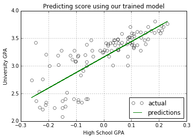

png

Supervising the Gradient Descent

There are several factors that will affect how GD converges, the learning step, the quality of the training data. It is useful to observe how GD behaves during training. One way to show how GD works is to plot the cost by the number of iteration to show if GD is decreasing the cost after each iteration. Here let’s do it.

In [12]:

def supervise_gd(model, X, Y, cost_derivative, rate=0.1, zoom=50):
    '''A helper function that plays with the training.
    
    zoom
        int, the word, think of it as a Lens observing our process
    '''
    costs = []
    optimizer = gd(model, X, Y, cost_derivative, rate, 1)
    for _ in optimizer:
        if len(costs) >= zoom: break
        cost = model.cost(X, Y)
        costs.append(cost)
        optimizer.send((rate, 1))
    return costs

In [13]:

def plot_cost(costs, learning_rate):
    plt.xlabel("i-th iteration")
    plt.ylabel("cost")
    plot(range(len(costs)),
         costs,
         'r-', antialiased=True,
         label="costs")
    legend = plt.legend(loc="upper right"
                       # fontsize='x-large', shadow=True
                       )
    # legend.get_frame().set_facecolor('white')
    plt.title("Gradient descent at learning rate %s" % learning_rate)
    plt.grid(True)
    plt.show()

In [14]:

model = LinearModel(np.ones(2))
zoom = 1000
learning_rate = 0.1
costs = supervise_gd(model, _X, _Y, cost_derivative, learning_rate, zoom)
plot_cost(costs, learning_rate)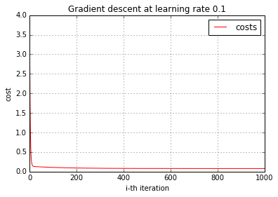

png

Let’s change our learning step and watch how that affects GD

In [15]:

model = LinearModel(np.ones(2))
zoom = 1000
learning_rate = 0.01
costs = supervise_gd(model, _X, _Y, cost_derivative, learning_rate, zoom)
plot_cost(costs, learning_rate)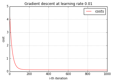

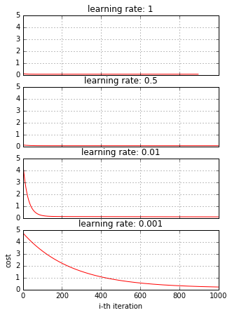
png

Here are a few more

In [16]:

def plot_cost2(data):
    f, axes = plt.subplots(len(data), sharex=True, sharey=True)
    plt.xlabel("i-th iteration")
    plt.ylabel("cost")
    for (i, (costs, learning_rate)) in enumerate(data):
        axes[i].plot(range(len(costs)),
                     costs, 'r-', antialiased=True)
        axes[i].set_title("learning rate: %s" % learning_rate)
        axes[i].grid(True)
    plt.show()

In [17]:

with zoom_plot(5, 7):
    plot_cost2([
            (supervise_gd(LinearModel(np.ones(2)), _X, _Y, cost_derivative, 1, 1000), 1),
            (supervise_gd(LinearModel(np.ones(2)), _X, _Y, cost_derivative, 0.5, 1000), 0.5),
            (supervise_gd(LinearModel(np.ones(2)), _X, _Y, cost_derivative, 0.01, 1000), 0.01),
            (supervise_gd(LinearModel(np.ones(2)), _X, _Y, cost_derivative, 0.001, 1000), 0.001),
        ])

png