Chaobin Tang (唐超斌)

Linear Regression with Multiple Features

In trying to understand gradient descent, I have built a linear regression model with one input, now I am taking that same model and generalize it to use multiple inputs. So an immediate question to construct this model is what inputs or features I am going to use. It turns out this question is a general question in machine learning. To decide the inputs for a model not only involves the domain knowledge, such as knowledge on the the credit in building a credit risk model, also involves many techniques learning useful information from the training data.

Feature selection

The many different models will all face one problem, that is to decide which feature to use. In the context of machine learning, this topic is called feature selection, or rather, feature engineering in large. In other context, it is also related to dimentionality reduction. It is often said that selecting the proper set of features is more important than fitting the parameters, as by training the model, we are only approaching the optimum of precision that is already determined by the feature set we introduced into the model. On the other hand, the inputs may also contain the irregularities or noises that could challenge the model’s ability to generalize. Therefore, it is rather important to investigate the feature set used in a model before the significant work is carried on training.

There are many techniques and algorithms we can use in feature selection, such as the wildly used Principle Component Analysis, as well as a connectionist approach called Restricted Boltzmann Machine which is now a building block in many deep learning architecture used for representation learning. The following will however, omitting further discussing on the topic, use a basic approach by measuring the correlation between the feature and outcome. The correlation measure used is the Pearson Correlation.

In [2]:

# Here I used pandas just to simplify the process
# of retrieving and preprocess data. I will then
# get the internal numpy narray to work with thereafter.
import math
import pandas as pd
from pandas import DataFrame, Series

URL_GPA = "http://onlinestatbook.com/2/case_studies/data/sat.txt"

def online_gpa():
    df = DataFrame.from_csv(URL_GPA, sep=' ', header=0, index_col=None)
    return df

df_gpa = online_gpa()
column_names = list(df_gpa.columns)
data = df_gpa.values

Pearson Correlation is based on measuring the variance of data(I found PCC a helper in memorizing several statistical equations as it combines several measurements into one single equation). Anyway, the Pearson Correlation gives you a linear correlation measure between two variables. In our case, this can be used to tell us the level of correlation (not causation, although a correlation sometimes leads to the discovery of causation, but usually it needs some domain knowledge or common sense to justify) between each input and the outcome.

In [3]:

# pandas has a corr() that by default uses the pearson method
# to calculate the correlation pair-wise.
# Here we do that and take the two most correlated
# columns out of the data and use them in our
# multivariate model.

features = df_gpa.corr()['univ_GPA'].sort_values(ascending=False)[1:3].index.tolist()
columns = [column_names.index(f) for f in features]

In [1]:

%matplotlib inline
from importlib import reload
from isaac.models import regressions
from isaac.pipeline import preprocess
from isaac.plots import basic as plots

Cross Validation - The model that goes beyong the training data

To think of machine learning as a way of producing a program by inputting data (versus producing a program by inputting source code), You want the machine learned program to be able to perform well not only on training data that helped train the model, but also make good predictions about the unseen data. For example, using a small portion of the user data on their preferences in music, you want the model to be able to predict the preferences of all your users and recommend music for them.

A model can be -

• underfitted, or biased, for parametric models such as the linear regression model I’ve built, it could be a result of using too few features that are unable to capture the relationship between input and output.
• overfitted, or variant, for our model this could be a result of using too many features that resulted an almost perfect fit to the training data, when applied to unseen data the model is producing very high variance.

In either case, the model will not be able to generalize. Apart from other techniques such as regularization, cross validation is one of them that should be applied in the earliest stage of the process.

Optimization algorithms such as gradient descent takes several parameters:

• the learning rate
• the lambda in the regularization term
• the batch size in stochastic gradient descent

The value of these parameters have direct impact on the model’s performance during training. And these parameters are called hyperparameters, in a sense that these parameters are different from those in the model yet also impact the performance of it.

Training a model is to fit the model’s parameters to the training dataset. One thing we want to make sure during training is to obtain a good balance between being overfitted and underfitted. We need a measure to tell us. A straightforward method would be to have it to make some predictions on unseen data. If the quality of prediction satifies us we can stop the training. Otherwise we shall continue tuning the model and perhaps adjust the hyperparameters such as learning rate so that the model’s cost continues to decrease. Here comes the point of cross validation: the unseen data should be the data set that is not used in any process of training, neither in fitting the model’s parameters nor used to tune the hyperparameters. So if we are given one data set X, using cross validation, we shall make three partitions out of X, one as training set, one test set to measure the prediction, and one as the unseen data to tell us how well the model is really doing on data it has never seen. One can think of the test set as the training set used to train the hyperparameter.

In [4]:

from sklearn.cross_validation import train_test_split

In [5]:

X, Y = preprocess.get_XY_from_frame(data, columns)
X_train, X_test, Y_train, Y_test = train_test_split(
    X, Y, test_size=0.33, random_state=42)

In [6]:

model = regressions.LinearRegression.from_dimension(len(features) + 1)

In [7]:

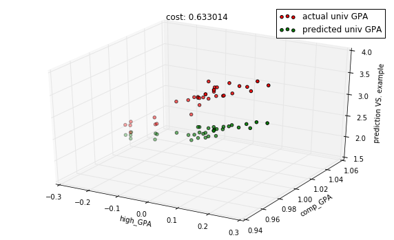
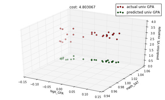
# the untrained, initialized model
predictions = model.predict(X_test)
cost = model.costs(X_train, Y_train)
title = "cost: %f" % cost
with plots.zoom_plot(10, 6):
    plots.plot_predictions_3d(X_test, Y_test, predictions, features, title=title)
    plots.plot_predictions_3d(X_test, Y_test, predictions, features, title=title, mirror=True)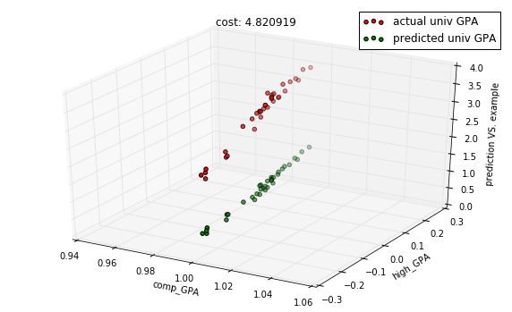

In [8]:

from isaac.optimizers import gradient
reload(gradient)

<module 'isaac.optimizers.gradient' from '/Users/cbt/Projects/isaac/isaac/optimizers/gradient.py'>

In [9]:

descent = gradient.Descent(model, X_train, Y_train, 0.001)

In [10]:

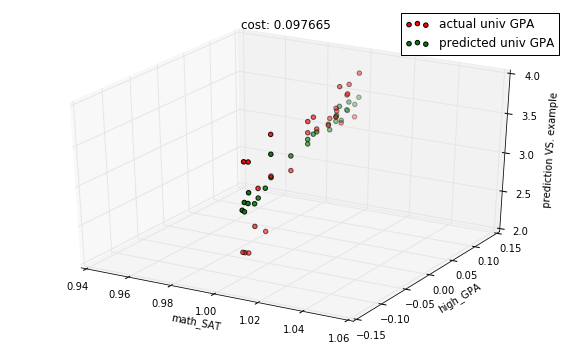
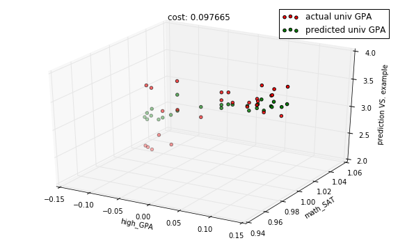
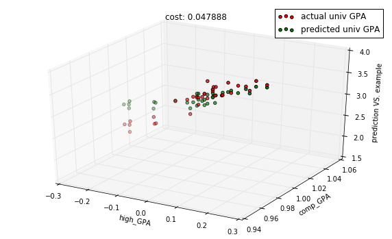
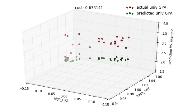
descent.run(10)
predictions = model.predict(X_test)
cost = model.costs(X_train, Y_train)
title = "cost: %f" % cost
with plots.zoom_plot(10, 6):
    plots.plot_predictions_3d(X_test, Y_test, predictions, features, title=title)
    plots.plot_predictions_3d(X_test, Y_test, predictions, features, title=title, mirror=True)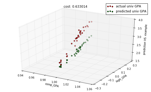

In [11]:

descent.run(50)
predictions = model.predict(X_test)
cost = model.costs(X_train, Y_train)
title = "cost: %f" % cost
with plots.zoom_plot(10, 6):
    plots.plot_predictions_3d(X_test, Y_test, predictions, features, title=title)
    plots.plot_predictions_3d(X_test, Y_test, predictions, features, title=title, mirror=True)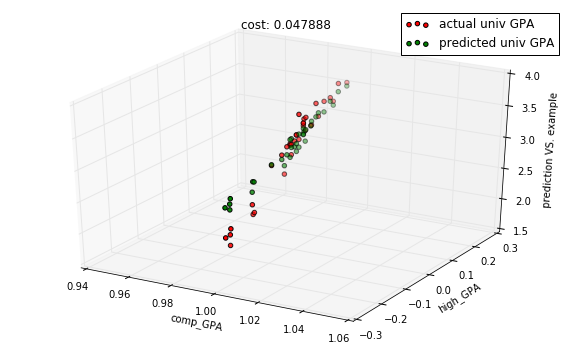

In [12]:

# Let's use the bottom ranked features and compare
# the model with one above

In [13]:

features = df_gpa.corr()['univ_GPA'].sort_values(ascending=True)[1:3].index.tolist()
columns = [column_names.index(f) for f in features]

In [14]:

model = regressions.LinearRegression.from_dimension(len(features) + 1)
X, Y = preprocess.get_XY_from_frame(data, columns)

In [15]:

X_train, X_test, Y_train, Y_test = train_test_split(X, Y)

In [16]:

descent = gradient.Descent(model, X_train, Y_train, 0.001)

In [17]:

# untrained model
predictions = model.predict(X_test)
cost = model.costs(X_train, Y_train)
title = "cost: %f" % cost
with plots.zoom_plot(10, 6):
    plots.plot_predictions_3d(X_test, Y_test, predictions, features, title=title)
    plots.plot_predictions_3d(X_test, Y_test, predictions, features, title=title, mirror=True)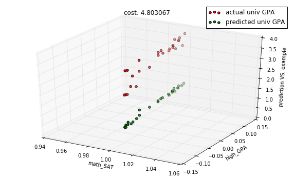

In [18]:

descent.run(10)
predictions = model.predict(X_test)
cost = model.costs(X_train, Y_train)
title = "cost: %f" % cost
with plots.zoom_plot(10, 6):
    plots.plot_predictions_3d(X_test, Y_test, predictions, features, title=title)
    plots.plot_predictions_3d(X_test, Y_test, predictions, features, title=title, mirror=True)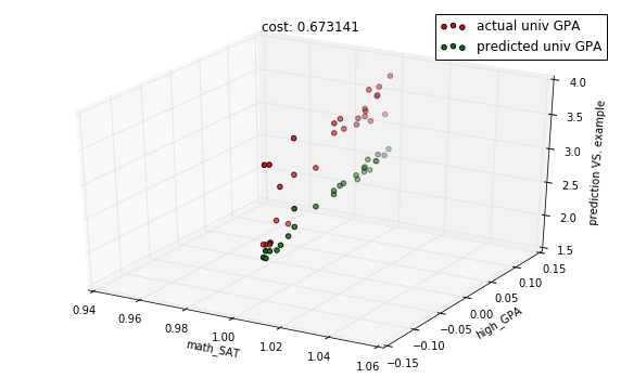

In [19]:

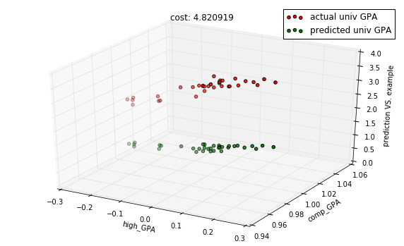
descent.run(50)
predictions = model.predict(X_test)
cost = model.costs(X_train, Y_train)
title = "cost: %f" % cost
with plots.zoom_plot(10, 6):
    plots.plot_predictions_3d(X_test, Y_test, predictions, features, title=title)
    plots.plot_predictions_3d(X_test, Y_test, predictions, features, title=title, mirror=True)