Chaobin Tang (唐超斌)

Understand and Build a Neural Network on Digit Recognition

The multilayer perceptron, is not only itself a very powerful statistical model used in classification, it is now a building block to some of the deep networks that made recent headlines. The understanding of MLP can rise from that of the logistic regression previously investigated, and will be essential to understand many 2016 deep neural networks. In this post, in addition to the mathematical reasoning that I accepted as being necessary, I am to provide an intuition that helped me a lot to grasp the back propagation algorithm. In the end, a classifier using everything in this post is built and tested on a task of recognizing hand written digits from images.

Representation - A generalization of logistic discriminant from two class to multiclass

The logistic discriminant function we previously built:

applies a non-linear transformation on the linear sum of the parameters θ and the input x. And we then rely on the ability of the sigmoid function to allow us to interpret the mapped output as the posterior probability P(C|x). For a classfication problem with two classes:

and

Then we derived from a likelihood function:

a cost function:

that allows us, through the optimization method such as gradient descent, to find the optimimal settings of parameters that maximizes the probability of observing the training data. Ultimately we obtained a model and a training method to allow us to use a set of training data (with labelled data) to classify unseen data point.

Having seen its ability to classify a two-class example in the income class prediction in that post, we are now motivated to generalize the model to work on multiple classes. A generalized form of the discriminant can look like this:

where y_k represents the posterior probability of observing class k given parameter which is a vector w. We than note for each class k, there is a parameter vector w_i that maps an input x to one of the classes k_j, so now we have a matrix of parameters W. This transformation structure can be graphically represented as below, after which we refer to this structure as the neural network (The name neural network certainly gave it a lot of theatrical capacity, but the principles in the field mostly are formed from statistics. Although it is sometimes inspired by the biological neural systems such as human brain.):

In [265]:

# This is used during converting this notebook
NAME_POST = '2016-04-15-neural-network-on-digit-recognition'

In [275]:

from importlib import reload
from isaac.plots import net as netplot
# reloading the code changes
reload(netplot)
with netplot.folder(NAME_POST): g = netplot.forward_net((10, 5))
g

The neural network above has two layers, the input layer and the output layer. The dimension of the input layer is decided by the dimension of the data. In computer vision, it can be the size of the pixel vector flattened from an image pixel matrix. In NLP, it can be a one-hot vector that represents a word in the vocabulary. The dimension of the output layer, in classification problem, can be the number of classes. In generative problem, such as the language model in NLP, it can be as the same dimension as the output (A language model takes an input a sentence, and outputs a sentence that represents the predicted next word for each word in the observation.).

A neural network in theory can take on an arbitrary number of layers, and we refer to the layers between the input and output layer the hidden layer. Here is an example of the network that has three hidden layers:

In [276]:

with netplot.folder(NAME_POST): g = netplot.forward_net((10, 9, 7, 5, 5))
g

Theoretically, more layers can encode more information. Each layer can pick up what’s encoded by the layer before it and learn the pattern from it. So, the latter layers can learn the pattern that is more abstract. Being attempting as it is, there are practical reasons that in real world people don’t use the neural network that has two many hidden layers. One of the problems corresponds to the fact that when training a neural network that has more than one hidden layer, it becomes increasingly difficult for a training method such as gradient descent to fine tune the weights of the earlier layer, resulting a dismatch of the performance one might expect from adding more hidden layers into the network. Recent progresses however in the field of deep learning most often involve networks that has many hidden layers, their successes are results of many cutting-edge techniques that were developed in the last decade or so that help overcome the problems from training such deep network. I will leave the investigations on these in other dedicated future post.

Forward propagation - computation of the neural network

In the plotted network above that has two hidden layers, the linear transformation on each layer takes place from left to right:

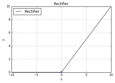
This is called forward propagation. When implemented in a vectorization library such as numpy, the computing is often to calculate a dot product followed by a nonlinear transformation g. The g is a choice of non-linear function such as the sigmoid function used in logistic regression. In neural network, the g is called an activation function (It should be pointed out that the hidden layers usually use the same choice of an activation function, while the output layer can use a different one.). Other popular choice of activation functions are:

tanh(x)

In [156]:

from isaac.models.networks import activations
reload(activations)
X = np.arange(-10, 10, 0.01)

In [163]:

Y = activations.Tanh.activate(X)
basic.plot(X, Y, style='k-', label="Tanh", title="Tanh",
                loc="upper left", show=False)
basic.plot(0, 0, style='bo')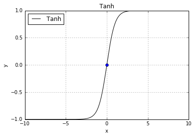

rectifier: g(z) = max(0, z)

In [162]:

Y = activations.ReLU.activate(X)
basic.plot(X, Y, style='k-', label="Rectifier", title="Rectifier",
                loc="upper left", show=False)
basic.plot(0, 0, style='bo')

(2000, 2)

Normalized sigmoidal output - retain the ability to interpret the result as the multiclass membership probability distribution

The above looks a natural generalization of the logistic regression from two class to multiclass. But an immediate problem arises in that representation is that the ability to interpret the result transformed by the sigmoid function as the probability distribution no longer holds true, because for classes C > 2:

where:

no longer lies in the range (0, 1). To retain the ability to interpret the result as the class membership probability distribution, we need to normalize the output function so that for mutually exclusive class membership, the sum of the output will add up to 1. The normalization is defined as:

This normalization is often called softmax, in the sense that it is a smoothed/soft version of the maximum sigmoidal output. It is also worth pointing out that in practice, the represetation will continue to function regardless of the output function being normalized or not. There is a difference beyond being more mathematically plausible however, that when using the softmax, the cross entropy cost function will feedback a more accurate cost thus alleviate the learning slowdown problem when the neural network saturates. The saturation of a neural network is best depicted by its sigmoidal output:

In [164]:

%matplotlib inline
from matplotlib import pyplot as plt
import numpy as np

from isaac.models.networks.activations import Sigmoidal
from isaac.plots import basic
X = np.arange(-10, 10, 0.01)
Y = Sigmoidal.activate(X)
basic.plot(X, Y, style='k-', label="sigmoid", title="Saturation: the change of x slows down at both ends",
                loc="upper left", show=False)
basic.plot(0, 0.5, style='bo')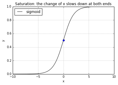

Cost - summing the cost of the prediction on each class

The cost of the generalized logistic regression on multiclass is nothing more complicated but summing all costs (in this case, the cross entropy cost is used) of the prediction on each class:

Motivation - why neural network?

One of the most important motivations is that the neural network can represent very complex decision boundary. Let’s look at some of the decision boundaries:

In [49]:

import random

from sklearn import datasets

from isaac.plots import basic
reload(regressions)
reload(basic)

<module 'isaac.plots.basic' from '/Users/cbt/Projects/isaac/isaac/plots/basic.py'>

In [96]:

n_samples = 5000
x, y = datasets.make_moons(n_samples=n_samples, noise=.1)
basic.plot_clusters(x, y, 2, basic.Palette.BLUE)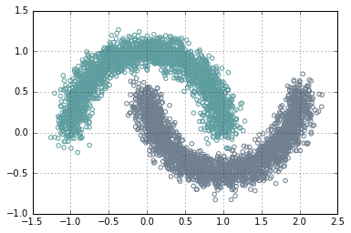

In [97]:

from isaac.models.clustering import kmeans
def cluster(k=2):
    model = kmeans.KMeans(x, k=k)
    converged, clusters = model.fit(20)
    basic.plot_clusters(x, clusters, k, basic.Palette.BLUE)

In [98]:

cluster(4)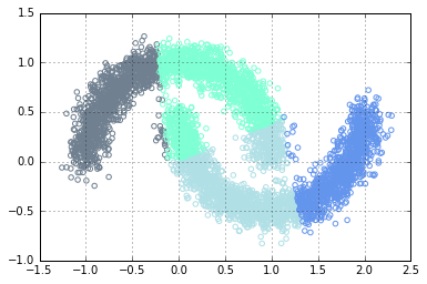

Using one-vs-all, the data above is still separable using logistic regression classifier.

In [116]:

cluster(10)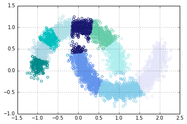

In the plot above, some shapes of the decision boundary is disjointed. It cannot be represented by a logistic discriminant.

Universality - A neural network with one hidden layer can compute any function

The ability as to what can be represented by a neural network and the configuration requirement was well studied. Using nonlinear activation, such as sigmoid function, a neural network with just one single hidden layer can represent an arbitrary decision boundary. (TO ADD: an intuition on constructing templates that compute boolean functions) An example with one hidden layer that has the same number of units as that in the output layer:

In [277]:

with netplot.folder(NAME_POST): g = netplot.forward_net((10, 5, 5))
g

We talked about the adaptation of the normalization of sigmoid function as well as the cost function in order for this generalized multiclass discriminant to work, now we focus on the adaptation on the training method, after which we will have completed building a new powerful model that can compute any function.

Back propagation - Using chain rule to propagate backward the changes of cost with respect to weights in each layer

The optimization methods such as gradient descent only needs one essential ingredient, that is a measure of the change of cost with respect to the parameters(weights). Analytically, that will help nagivate the weight search to locate the optimal values of weights that give the least amount of aggregated error on observations. Compared to what we have done in logistic regression, a new problem arises that now we have parameters that control the hidden layers that are not directly connected to the final output. In other words, the weights of hidden layers will have to be calculated intermediately.

Chain rule - Marry is twice faster than Linda, and Kathy is twice faster than Marry, then how faster is Kathy than Linda?

The answer to that question is simple, Kathy is four times faster than Linda. This is an intuitive and true understanding on the chain rule, which formally states:

Given y = f(u), u = g(x), when f is differentiable in u, and g is differentiable in x, then the definition:

is differentiable in x, and

or

In plain terms, this allows us to compute the rate of change with respect to the variable that is indirectly influencing the function. Applying the chain rule, when we want to do that, we can find an intermediate relationship between the indirect variable and the function, then calculate two simple derivatives and multiply them to give us the measure of rate of change of the function with respect to the indirect variable.

Let’s begin

Because when we calculate the rate of change of cost function with respect to the weights in each layer, we start with the cost function which is the aggregation of the output of the final layer:

we are walking backward to calculate the weights layer by layer. It should become clear now why this algorithm is called back propagation. Instead of directly calculating the cost-weight Jacobian matrix, the back propagation algorithm involves calculating an intermediate measure called δ, and takes the following steps for each iteration:

The back propagation of the intermediate measure δ runs in the opposite direction of forward propagation, doing the calculation defined by the equations above:

In [278]:

with netplot.folder(NAME_POST):
    g = netplot.forward_net((10, 5, 5), labels=('input', 'hidden', 'cost'), reversed=True)
g

1. The first equation is the hadamard product in the final layer L of these two results:

   • partial derivative of cost with respect to activation
   • the derivative of the activation with respect to neuron input of final layer

   For one single training example, the result of this step is a vector whose size is determined by the number of output neurons in the final layer.

2. The second equation is another hadamard product in the layer L-1 earlier than final layer of these two results:

   • the dot product of the weights in layer L-1 and δ in layer L
   • the derivative of the activation in layer L-1 with respect to neuron input of layer L-1

   For one single training example, the ressult of this step is a vector whose size if determined by the number of neurons in layer L-1.

3. The third equation calculates our target value, the partial derivative of the cost C with respect to the weight in the layer. It needs to be pointed out this is an outer product of:

   • the activation in the input layer L-1
   • the δ in the current layer L

   For one single training example, the result of this step is a matrix m x n, where m is the number of neurons in layer L, and n is the number of neurons in layer L-1

Intuition - Contribution to the final error C, when back propagated, is first distributed on each neuron by their weights, then distributed on each weight by the input

I always seek an intuitive understanding, or at least, an intuitive transformation of understanding to try to understand complicated processes. The simplification above is the one that I think makes sense to me and worked quite well in grasping the very essentials of the back propagation algorithm. Two important calculations happen during propagation:

1. Distribute δ of layer L to the neurons in layer L-1 the proportion decided by the weights of neuron in L-1. The dot product between the weights and δ reflects this.
2. For every neuron in L-1, further distribute the δ to each weight inside one single neuron based on the activation it receives from the layer before it. The outer product between the activations and δ in current layer reflects this.

Chain rule - Here is how the back propagation is derived mathematically by applying the chain rule repeatedly:

The ultimate goal is get the partial derivative of cost C with respect to each weight w in each layer l. The following equation applies the chain rule twice to measure this indirect relationship between the variable w and cost function C:

Code - Putting everything together to build a hand written digit recognizer

The code used below is from a project I put together during study and can be downloaded from here:

$ git clone https://github.com/chaobin/isaac.git
$ git checkout nn # the branch that this post uses

In [210]:

%matplotlib inline
import numpy as np

In [211]:

from importlib import reload # used to modified code changes

In [212]:

from isaac.models.networks import forward
from isaac.models.networks import activations
reload(forward)
reload(activations)
from isaac.pipeline import preprocess
reload(preprocess)
from isaac.plots import basic

A helper function that displays the mnist data as an image:

In [213]:

def show(img, shape, title=''):
    """
    Render a given numpy.uint8 2D array of pixel data.
    """
    img = img.reshape(shape)
    from matplotlib import pyplot
    import matplotlib as mpl
    fig = pyplot.figure()
    ax = fig.add_subplot(1,1,1)
    imgplot = ax.imshow(img, cmap=mpl.cm.Greys)
    imgplot.set_interpolation('nearest')
    ax.xaxis.set_ticks_position('bottom')
    ax.yaxis.set_ticks_position('left')
    pyplot.title(title)
    pyplot.show()

The mnist data set is an open database of handwritten digits. Also, I am using python- mnist, a Python library to parse and load the mnist data. The mnist data comes in with two sets, the training set that contains 60,000 images, and the testing set that contains 10,000 images.

As with all machine learning applications, there are quite many things to be done to the data. Here the preprocess include:

• scaling the pixel values by 1/255
• converting the labelling to a one-hot vector

In [214]:

PATH_MNIST = "/Users/cbt/Documents/research/"
# loading raw data
train_images, train_labels = preprocess.load_training_mnist(PATH_MNIST)
# scaling color intensities, converting integer labels into 10-bit bitmaps
train_images, train_labels = preprocess.training_mnist_preprocessed(PATH_MNIST)

Generalize - Use one part of training data to tune hyperparameters

There will be dedicated posts on generalization in the future, but right now I will use the cross validation by splitting my training data into two batches.

In [215]:

from sklearn.cross_validation import train_test_split
train_images, validate_images, train_labels, validate_labels = train_test_split(train_images, train_labels)

The testing data set will only be used for testing the trained network.

In [216]:

test_images, test_labels = preprocess.load_testing_mnist(PATH_MNIST)
test_images, test_labels = preprocess.testing_mnist_preprocessed(PATH_MNIST)

In [217]:

with basic.zoom_plot(2, 2): show(test_images[15], (28, 28))

The architecture of a network refers to the configurations, such as the number of layers, number of neurons in each layer, the activation function in hidden layers, and the activation function in the final output layer. Here below the vanilla network I constructed for this purpose has three layers. The input layer is determined by the input image vector, each neuron will encode one pixel. The output layer corresponds to the one-hot vector that represents the label of the image. The hidden layer, however, is using an experimental 50 number of neurons. There is significance in choosing a different number of neurons such as this one, but I will omit the discussions on this here.

So our network will take as input a vector flattened from the image matrix, its element will be the pixel value scaled into the range (0, 1). And the network will output a vector of length 10, whose elements represents the probability of the neuron being the digit that corresponds to the nenron’s place in the final layer.

In [224]:

num_features = train_images.shape[1]
layering = (num_features, 50, 10)
mnist_net = forward.Network(layering)

The initial cost

In [219]:

mnist_net.cost(validate_images, validate_labels)

16.907340009640887

The initial accuray (Since the newly constructed network’s weights is pretty much randomly initiated, we should expect that its prediction on the digit is like making an uneducated guess that is close to be 1 out of 10):

In [220]:

mnist_net.accuracy(validate_images, validate_labels)

0.078200000000000006

Train the network with stochastic gradient descent using an experimental learning rate 4.0, and 100 for batch size, and 30 epochs (It should be pointed out that I chose these values during my experimentation on the basis that they worked out achieving the expected accuracy within reasonable time. I talked about the relationship between the learning rate and the convergence behaviour of gradient descent previously, but haven’t done so for the stochastic gradient descent as well as the batch size of it. These parameters and their effects on the algorithm are also well studied. To sum what I have read from the papers on SGD, SGD will not only converge nonetheless when fed with one single training set in each iteration, importantly it is also likely to escape a local optimal and find a globally better optima in the weight space. The choice of the batch size, if kept too large, will compromize this ability to the extent when the size is as large as the entire training data that is no different from the standard batch gradient descent; when too small on the other hand, will cause the algorithm to take longer to converge. The practitioners will find themselves experimenting with these settings in many applications as said by many people, although there exists automated control (such as simulated annealing on learning rate) of these settings and I will leave those in future posts):

In [221]:

mnist_net.SGD(train_images, train_labels, 4.0, 100, 30)

Epoch 0 completed.
Epoch 1 completed.
Epoch 2 completed.
Epoch 3 completed.
Epoch 4 completed.
Epoch 5 completed.
Epoch 6 completed.
Epoch 7 completed.
Epoch 8 completed.
Epoch 9 completed.
Epoch 10 completed.
Epoch 11 completed.
Epoch 12 completed.
Epoch 13 completed.
Epoch 14 completed.
Epoch 15 completed.
Epoch 16 completed.
Epoch 17 completed.
Epoch 18 completed.
Epoch 19 completed.
Epoch 20 completed.
Epoch 21 completed.
Epoch 22 completed.
Epoch 23 completed.
Epoch 24 completed.
Epoch 25 completed.
Epoch 26 completed.
Epoch 27 completed.
Epoch 28 completed.
Epoch 29 completed.

In [222]:

mnist_net.cost(validate_images, validate_labels)

0.39948210538076773

After the training, the network is able to produce a 95.1% accuracy.

In [223]:

mnist_net.accuracy(validate_images, validate_labels)

0.95073333333333332

What’s next

Though at first it looks impressive when to think a computer program can derive that pattern out of the data without being explicitly programmed by human with the knowledge to recognize a hand written digit, the accuracy of 95.1% leaves 4.9% errors which has been the very dynamic to many advancements in recent years in neural network. There are many techniques, I would prefer to say, that were theoretically formalized and in practice validated that have made impressive success pushing the boundary of that 4.9% to a new limit. In the next post, I will dive into one of the techniques called Convolutional Neural Network that was particularlly effective on recognizing patterns in image.

References

Neural Networks for Pattern Recognition by Christopher M. Bishop